Our garage has a slightly weird, curvy bit of concrete around which needed to fit a piece of straight guttering. Although it could almost be bent into shape, I decided the neatest way to go about it would be to cut 1 or more wedges in the piece of guttering so that it wraps around the concrete nicely.
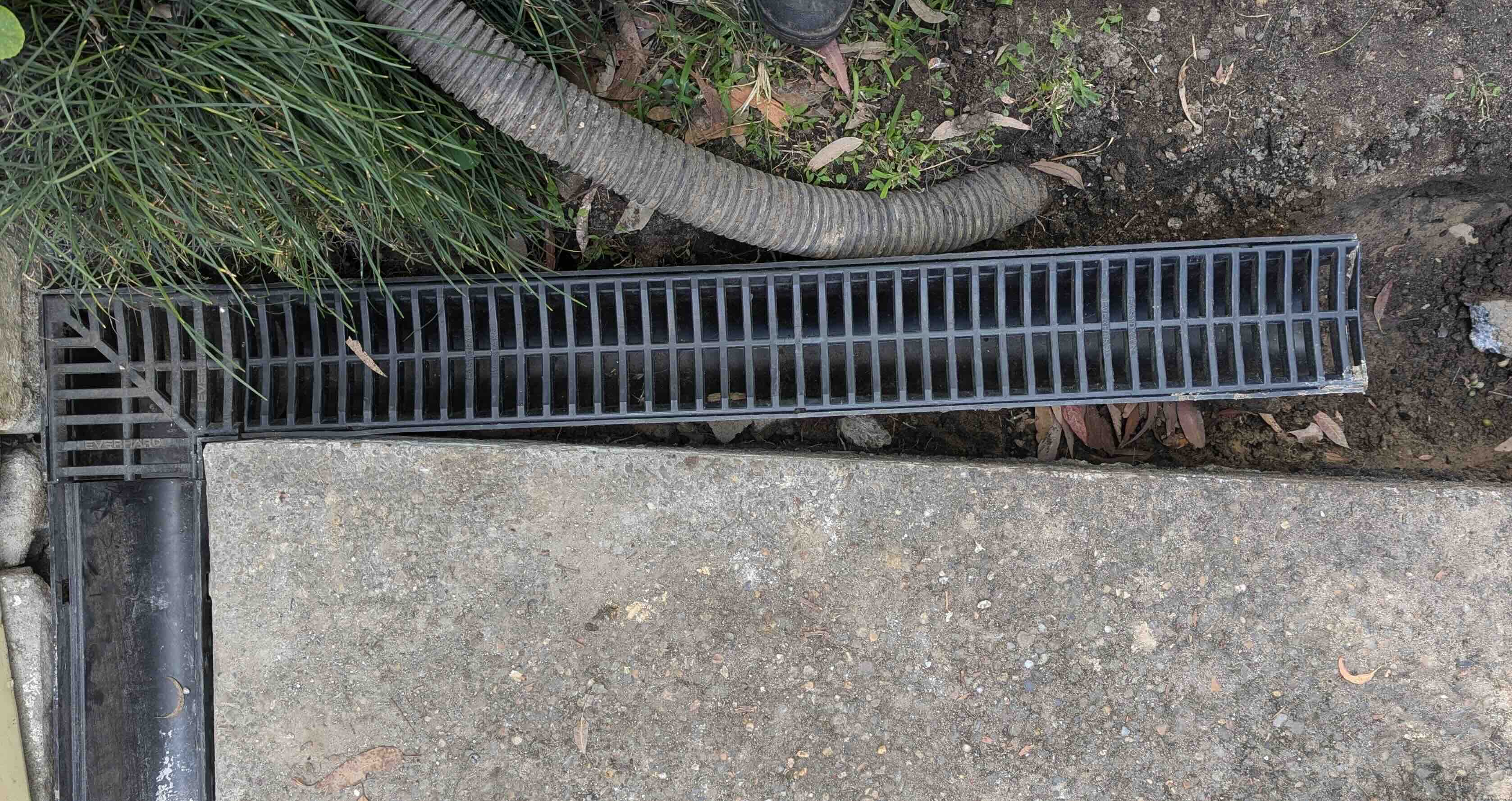
Thus the problem is deciding how many times to cut, where to cut, and at what angle? The quick and dirty (and quite valid) approach would be to estimate and measure it physically with a couple of rulers. But, being a software engineer, I was inclined to figure it out virtually, for the benefits of precision, flexibility and an objective measurement of how good the fit was for an increasing number of cuts!
For a brief moment I thought about just manipulating the image in Photoshop to align the guttering by hand, but saw it becoming a tedious and unfulfilling exercise in Photoshop skills. Having recently brushed up on a lot of mathematics, and learnt about Lagrange multipliers and constrained nonlinear optimisation, I saw that this was a great opportunity to put this knowledge into practice. Even though the layperson could easily argue that it was overkill, the mathematical formulation seemed quite straightforward in my head, so I could find a general solution, and it would only take me a few hours to code up, right? Surely??
As with all good problems, it took quite a bit longer, but I learned a lot on the way! Here’s how it went down, using Python.
Fitting a curve
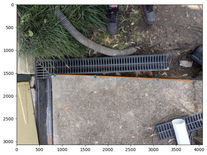
The first step was to define the curve that the concrete takes. The simplest way to do that was just mark the points by hand (I found a simple way to do it with an interactive figure thanks to ipympl). Make sure to rotate the image so that the start point is leftmost, and that the curve is a function of x (i.e. horizontal and does not double back on itself). Initially I was going to fit a spline, but the extra complexity of having a piecewise curve was unnecessary, and a cubic polynomial was absolutely sufficient.
The cubic needs at least 4 points to be defined, and the coefficients are easily obtained with np.polynomial.Polynomial.fit. Here is a plot of the resulting curve:
Objective function
The next step was to define the objective function, i.e. the function we are trying to minimise. Here, it is obviously the area between the gutter segments and the curve we want to minimise - we want the guttering to fit as closely to the curve as possible.
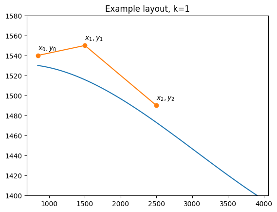
This means we just need to integrate the distance between the line segments and the curve. We’ll define each line segment by its endpoints with coordinates $(x_0,y_0), (x_1,y_1)$. The integral for a single segment looks like:
\[F_0 = \int_{x_0}^{x_1} \underset{\text{line segment}}{\underbrace{\frac{y_1-y_0}{x_1-x_0}(x-x_0)+y_0}} - \underset{\text{curve}}{\underbrace{(ax^3 + bx^2 + cx + d)}} \ dx\]Across multiple segments, all we need to do is add up this expression evaluated for each segment (a piecewise integral). Thus the other important parameter for the problem is the number of cuts, $k$, resulting in $k+1$ segments, and our full objective function can be expressed as follows:
\[F^* = \min \sum_{i=0}^{k+1} \int_{x_i}^{x_{i+1}} \frac{y_{i+1}-y_i}{x_{i+1}-x_i}(x-x_i)+y_i - (ax^3 + bx^2 + cx + d) \ dx\]Because we have a nice, analytical expression for this objective, we can help out our optimisation algorithm find its minimum by providing it with the analytical Jacobian (gradients). This just involves taking the partial derivative of the expression with respect to $x_0$, $x_1$, $y_0$, and $y_1$.
Now, the computation of this integral and the partial derivatives is fairly straightforward with some high-school calculus, but it gets a little unwieldy with so many terms. So after going through the motions, making a few small errors, and looking ahead to the multi-segment version and the future constraints that I was going to have to define, it was going to be much quicker and more flexible to get the computer to do this tedious work for me. So, thanks to the symbolic maths package SymPy, all the calculus and analytical expressions could be obtained with easy one-liners, and with full confidence of no silly mistakes. Wonderful!
Constraints
This part took the longest to get right. I started by making sure I could calculate the answer for a single segment, before expanding to multiple.
The easy constraints were:
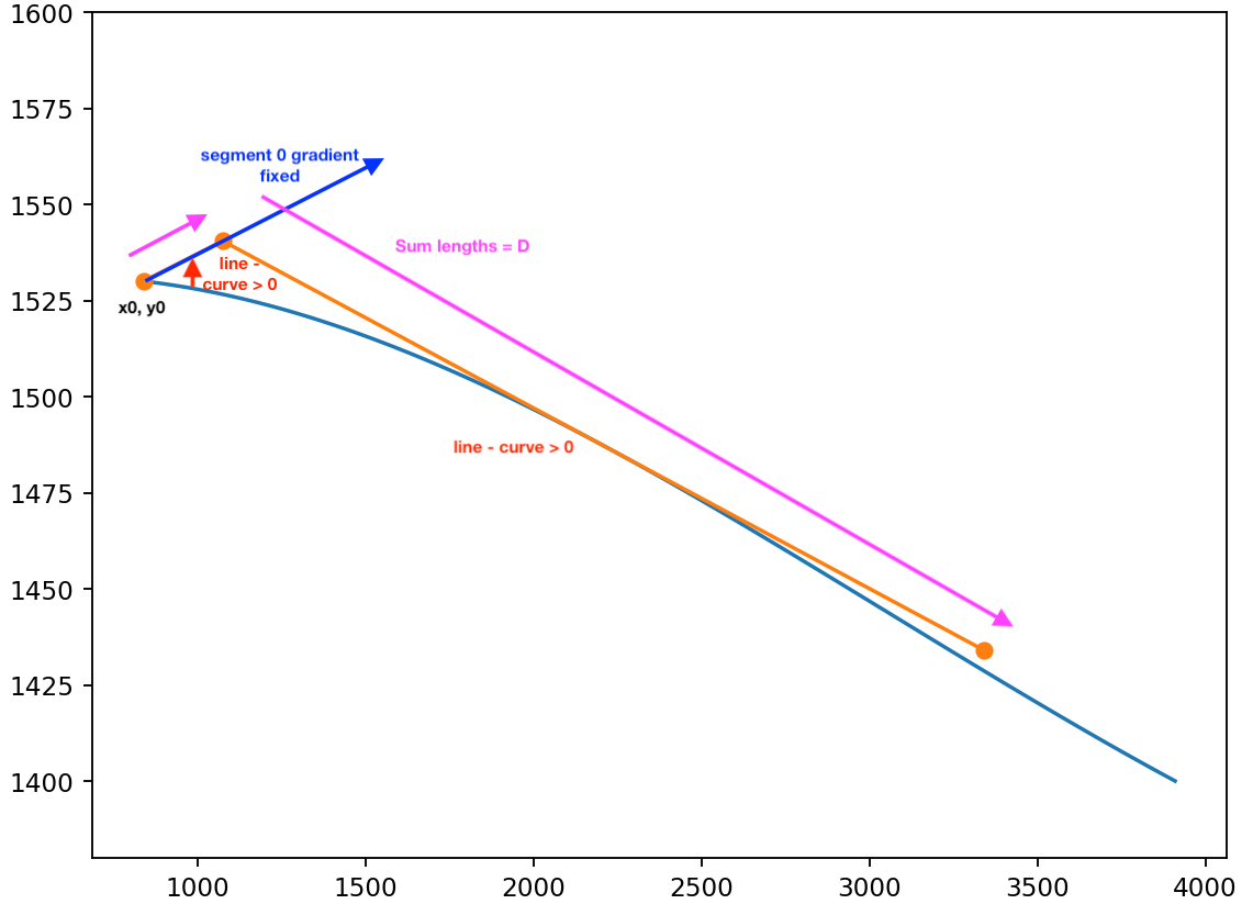
- The start point $(x_0, y_0)$ was fixed
- The first segment’s gradient is fixed, as determined by the fixed joint where the guttering piece we’re cutting meets the right angle piece on the left.
- The total length of the segments is equal to the original length of the guttering, $D$. I decided not to model the small change in length from cutting an angled segment in the guttering, for simplicity. SymPy was invaluable in computing the Jacobian for this constraint across all segments.
The constraint that proved to be a little more tricky to define, was that each line must always lie above the curve.
Initially, I thought that simply constraining each cut $(x_i, y_i)$ to lie above the curve, and have a gradient greater than the curve at that point, would be enough. This does indeed ensure the line never crosses, but after testing I quickly realised it prevented the optimal solution - in the case where the first cut would lie above the curve by some distance, the next cut may need to come down lower to meet the curve, requiring a lower gradient than the curve beneath. (e.g. look at $(x_2,y_2)$ in the example layout figure above - the gradient of the second segment needs to be steeper than the curve so that the endpoint can hug the curve).
My next idea was to find points of intersection between the line segment and the curve, and if any intersections occur in $ x_i < x < x_{i+1} $, the constraint is violated. With a cubic curve, these intersections can be computed analytically by finding the roots of the equation. However, this doesn’t play nicely with the solver as it is a discontinuous function with no gradient - either False for an intersection or True for no intersection, making iteratively finding the border of this constraint a challenge for the solver (we’ll get more into different solvers in a bit).
Thus my final idea was to calculate the minimum distance between the curve an the line. If the minimum distance is positive, the line is above the curve everywhere. This function is also continuous while the minimum lies between the segment bounds, so the solver has some idea of whether we’re approaching the curve and how close we are. Unfortunately, though, there are discontinuities due to the boundary condition at the line segment ends, and while I think it is possible to come up with an analytical solution, the discontinuity at the bounds means the derivative is undefined there. Thankfully, the solver was able to deal with this successfully (using its own finite differencing techniques for derviative estimation), and I didn’t need to worry about computing the Jacobian myself.
I did need to implement the computation of the minimum distance, however, for which I had two candidate ideas. Either sample a fixed number of points (say 100) along the line and choose the minimum, or run another iterative minimisation to find the minimum more precisely. I decided the latter, a bounded iterative minimisation, would be more efficient (it seemed to take around 1-3 iterations for each segment), more accurate, and better conditioned as the former discrete sampling method might introduce small discontinuities.
Improving the constraints
It took some playing around with the constraints to get the solver to converge successfully, and on the global minimum.
I found the solver converged more quickly and more stably with the constraint that each cut $(x_i, y_i)$ must lie above the curve. Although this constraint technically is already covered by the minimum distance constraint, its inclusion produced a definite improvement in convergence, and it is very simple to define along with its Jacobian.
Initially I hardcoded $x_0$ and $y_0$ in the calculations (as this point is fixed), but it meant I had to treat the first segment differently from the others in the code, whose x and y points were variables. It made the code a bit cleaner to instead have $x_0$ and $y_0$ as variables, and just add extra constraints on the solver to fix $x_0$ and $y_0$, and also potentially more extensible to future cases where this constraint was not wanted. This actually resulted in a conflict sometimes occuring between the minimum distance constraint for the first segment and the $y_0$ constraint, as the minimum distance occurs at $x_0$, but (presumably due to numerical errors) they would sometimes differ very slightly and cause the solver to throw an error, or prevent it from finding a good solution.
One solution was to relax the $y_0$ constraint to be an inequality, with $y_0<\delta$, $\delta$ being some small distance above the line. But what resulted in best convergence, was to keep the $y_0$ fixed constraint, and just remove the minimum distance constraint for the first segment. This minimum distance/line above curve constraint is basically taken care of by the other constraints of fixed gradient and $y_0$ and $y_1$ above the curve (at least, for the problem at hand), so could be safely removed for better convergence.
Solver
SciPy has 4 options for constrained minimisation, SLSQP, COBYLA, trust-constr, and COBYQA. Unfortunately they all have slightly different interfaces, making them a bit of a pain to test, but I did, yet could only get good results from SLSQP. I did have a brief flick throught the TRIP paper that trust-constr is based on, and played with some of the parameters, but could only get a clearly suboptimal result, and a deep dive on understanding the algorithm was beyond the scope of this project. COBYQA yielded an identical suboptimal result.
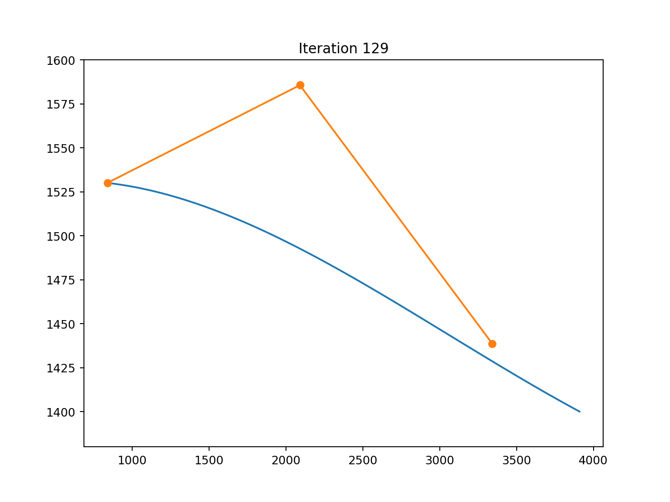
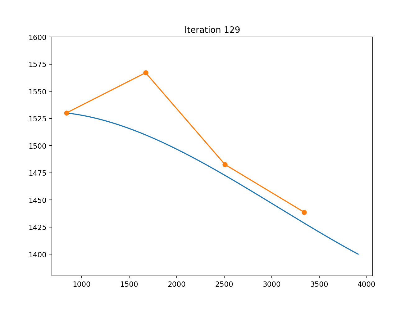
trust-constr and COBYQA, for k=1 and k=2. COBYLA couldn’t deal with equality constraints, so I forewent it.
But here are some nice videos of SLSQP converging on a couple of different solutions.
Because SLSQP is a quadratic programming solver, it starts to break down the further away from quadratic the problem gets. Take the following examples, which do not converge on a solution.
In this case, the solvers found in the mystic package would do a better job. I didn’t have the time to try it out, but had I known about the package, I would have started with it!
Results
Here’s a plot of the solution, for different numbers of cuts. With k=0 cuts the error is $243,105px^2$, with k=1, $8857px^2$, and with k=2, $2280px^2$, so we get a better fitting curve with more cuts, as expected. Converting to real units from pixels is a simple matter of measuring the length of guttering in real life. 1 cut looks like the way to go for me!
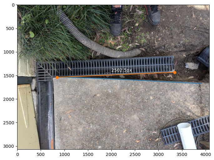
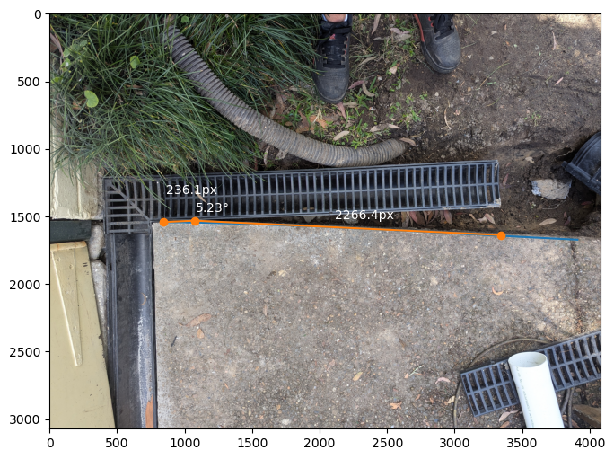

I’ll update it soon with the finished job :)
Code
A Jupyter notebook with the code is available on GitHub here.
